Hyperspectral data of clay minerals
|
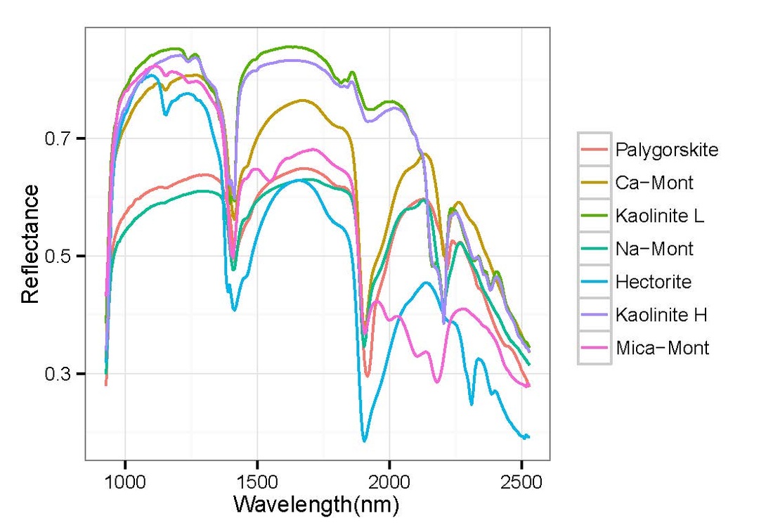
Powder samples of clay minerals (Fig.4) were scanned by the imaging spectroscopic system "sisuROCK" from SPECIM Ltd. The reflectance of these minerals were collected in the Short-wave Infrared (SWIR) wavelength (0.97-2.5 um). The hyperspectral data consist of 63 spectra (Fig. 5, left) of minerals with 256 bands. The 7 mineral types are represented by the averaged spectrum from 9 spectra for each type( Fig. 5 right).
Clay minerals are critical to mineral exploration but they are very identical with each other. They can be apparently distinguished by geochemistry analysis such as X-ray diffraction (XRD), yet the process is complex. Imaging spectroscopy facilitates the discrimination in the aspects of effort and economic saving. And the significance of band selection for mineral mapping is highlighted for the purity and similarity of these samples. Furthermore, the tool of "spatial and spectral endmember extract (SSEE)" in ENVI/IDL software is utilized to extract the purest endmembers for test. An endmember in mineralogy is a mineral that is at the extreme end of a mineral series in terms of purity (Wikipedia definition). Therefore, 43 test data were extracted by SSEE on each mineral type. And the mineral abundance of test data is assumed to be 1. |

Figure 4. Clay minerals
|

|
|
Figure. 5 Spectral data (left) and representative spectra of 7 mineral types (right)
Data exploration: CART
|
To ensure that the spectral data are correctly classified for RF analysis, we apply a classification and regression tree (CART) on the 63 spectra. Hyperspectral bands are regarded as predictor and mineral types are the response variables. CART aims to find groups of similar observations as the cluster analysis, .
The low error of the classification result indicates that the data are separated ideally according to the mineral type (Fig. 6, A-F represent 7 minerals). No mineral type is misclassified, which means these minerals are easily identified through multivariate statistics. Accordingly the RF analysis below which is based on CART will be slightly impacted by error arisen from the original data. |
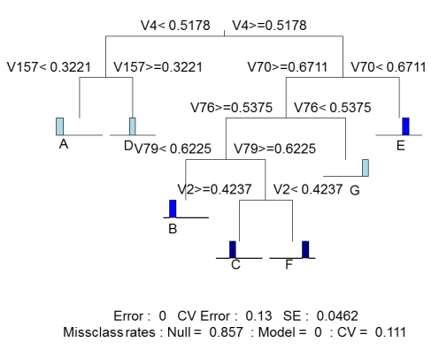
Figure 6. CART analysis
|
